
VOLUME 4: Table of Contents
TEACHING ISSUES AND EXPERIMENTS IN ECOLOGY
The experiment is conducted in our General Biology for non-majors class. This laboratory activity follows evolution and is conducted during the week of ecology. In class, students have received general instruction about ecological concepts, including niche, predation, aposematic coloration, crypsis, predator-prey interactions, and population growth. In the laboratory, students are introduced to the topic by being shown pinned insect predator and prey types (from a large collection maintained at the University). As the specimens of insects are discussed, a simulation of feeding appendage also is introduced. Note, we show a number of insects, including mandibulate predators (ground beetle, ladybird beetle, tiger beetle, predaceous diving beetle), predators that use raptorial forelegs (preying mantis, ambush bug, assassin bug, mantisfly), and predators that use all six legs (flying predators including dragonflies, damselflies, and robberflies). Additional photographs of many insect families are located at the Virtual Insect Collection (http://entomology.unl.edu/lgh/insectid/Virtual_insect/home.html). Insect predators are found in Diptera: Asilidae, Neuroptera: Mantispidae, Odonata (all), Hemiptera: Phymatidae). In addition to the specimens, the students are shown the illustration of feeding appendages that they will use (see Description: Figure 1).
Next, we discuss prey types and predation. Students are asked to think about prey defense strategies. These include camouflage (we show stick insects, plain grasshoppers, and thorn insects), aposematic coloration (we show wasps [Hymenoptera: Vespidae and Apidae], bright grasshoppers [Orthoptera: Acrididae], bright tiger moths [Lepidoptera: Arctiidae]), flash coloration (we show grasshoppers [Orthoptera: Acrididae] and underwing moth specimens [Lepidoptera: Noctuiidae]). As an alternative to pinned specimens, students can be shown images. In particular, an excellent source of images of many types of insects can be found at BugGuide.net (http://bugguide.net/node/view/15740). We discuss the steps of predation from search, identification, capture, and handling. We then point out insects that have defenses against all of these steps in the predation process.
During the introduction and ensuing discussion of prey defenses, we discuss poisons. Students are asked where insects obtain poisons and why not all insects are poisonous. During the fall term, live insects, including ladybird beetles and blister beetles are shown (both possess reflex bleeding and can be shown defending themselves). During spring semester, we show PowerPoint slides of bombardier beetles and monarch butterflies. The discussion is facilitated to ensure that the topics of evolution (acquisition of defense) and response to predation pressure are covered. We also discuss how a predator recognizes or "knows" if a prey item is poisonous. We show slides of the blue jays regurgitating after eating a monarch. We then talk about praying mantises doing the same thing when eating chemically defended prey.
In this exercise, students use a variety of feeding appendages constructed from plastic utensils (see Description: Figure 1) as they search the environment grabbing prey items (i.e., candy) and placing them into their stomachs (i.e., paper cups). For our simulations, we place equal numbers (n = 200) of three kinds of candy (M&M's, candy corns, and Skittles) onto shag carpet samples in a 2 x 3 m area. Candy represents edible prey and provides a handy snack at the end of lab; however, three or four types of small items, such as beans, buttons, plastic insects, etc., could also be used. Likewise, instead of using shag carpet to simulate a heterogeneous environment, the environment could consist of a grassy lawn (here, wrapped candy would be a must), a tabletop, or a cardboard box filled with packing material.
The instructors then assign feeding appendages based on these predator types and provide small paper cups that represent stomachs. Feeding appendages consist of pairs of plastic forks, knives, and teaspoons that are rubber-banded together to form a chopstick-like apparatus. The pairs of knives represent mandibles, pairs of teaspoons represent raptorial legs, and pairs of forks represent grasping legs. An equal number of each predator type is randomly assigned among the students (see Description: Figure 1).
Below are the rules that we use in the game. In our experience, non-majors have difficulty determining the rules based on ecological concepts. As a result, we have found it more useful to provide students with the rules and then discuss the ecological concepts related to those rules. However, in more advanced courses, students might be asked to determine the rules for foraging, learned avoidance, predator reproduction, prey reproduction, and the evolution of poisonous prey and predators that can eat them. With this approach, a guided inquiry could be used such that students are guided to the rules outlined below. It also may be possible to divide the class into smaller groups and have each group play the game with their own set of rules. Then, the groups could report back to the class in the form of a poster session or oral presentations to discuss how the rules they chose led to the results they found. Students at all levels could be asked to calculate the predator ratios and prey densities in the next year based on the rules. Although this step might increase the amount of time that it takes to complete a given game, it reinforces quantitative skills and increases student understanding of the dynamics of the game.
Potential Concerns and Questions: Make sure that predators are represented in approximately equal numbers. Students may wonder how they will know that a given prey item is poisonous. Mention that after 30 seconds if they eat something poisonous they will be informed of feeling ill.
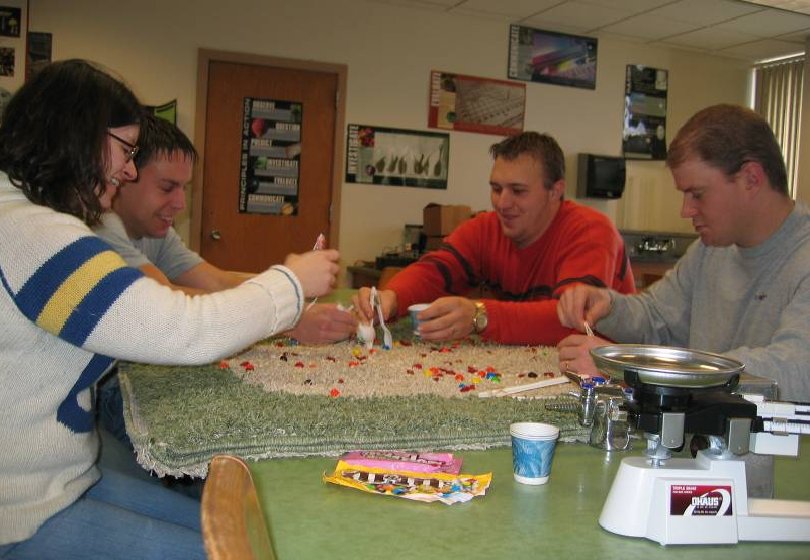
Students foraging on prey items on a table-top shag carpet environment.
Potential Concerns and Questions: It takes a long time to count individual prey items that were consumed. To speed this process, students sort their prey by kind into different cups and use balances to weigh each type. This way the number of prey of each type that has been consumed can be calculated quickly.
Based on the number captured, the number of prey remaining in the environment per species is calculated (200 - # eaten = # surviving) and prey are allowed to reproduce according to the following formulae. The poisonous species of the first round produces one copy of itself for each member that remains in the environment (doubles the number in the environment). The species that will remain palatable to all predators throughout the exercise reproduces at a rate of three individuals for each that remains in the environment. The other species will become unpalatable in the second round. It reproduces at an intermediate rate of two individuals for each that remains in the population.
In the second generation of the exercise, a second prey type becomes poisonous and cannot be eaten by any predator. Often, predation rates cannot keep pace with reproductive rates of some prey species. To avoid saturating the environment with prey (and to simultaneously maintain reasonable costs), a limit to reproduction by prey is imposed. Typically, no more than 300 prey per generation are added to the environment.
Potential Concerns and Questions. Students may question why there is a population cap on each species. This cap is explained ecologically as the role of intraspecific competition for resources (or environmental carrying capacity for a species). In the absence of predation, herbivorous species will increase in number until their food becomes limiting; then, only those members of the species that are able to acquire sufficient nutrients will be able to reproduce. In this exercise, each prey species is assumed to feed on different resources and thus is unaffected by interspecific competition.
Potential Concerns and Questions. Students also wonder how the number of predators are established for the next round. The predator numbers change in response to foraging success. Foraging success for each predator type is calculated and the reproductive success and thus reproduction is determined as the ratio of each predator type's success divided by the total prey consumed by all predators (e.g. amount eaten by P1/ amount eaten by (P1 + P2 + P3). The ratio of predators is adjusted by changing foraging morphologies of unsuccessful predators into those of successful predators at the appropriate frequencies.
Potential Concerns and Questions. Students wonder how a given predator type is chosen to adaptively detoxify the poisonous prey species. The predator type is chosen either at random or to favor the predators with the least members by the laboratory instructor. That predator type is able to eat all prey types except the prey species that becomes poisonous in the next round. The other predator types must selectively avoid both the poisonous prey type from the previous round and the new poisonous prey type as they struggle to overcome competition and reproduce.
Potential Concerns and Questions. Students will ask when the exercise is completed. The exercise is continued until stability is reached or all but one predator type or prey type has become extinct. A short discussion is conducted as the prey are replaced in the environment. Predictions about the community's behavior are made and the exercise is repeated as above again randomly assigning poisonous prey and predator adaptations.
Potential Concerns and Questions. Students at first are confused that they input mass into the spreadsheet (Excel® predpreyblank.xls (29k)) whereas the graph output is in numbers of individuals. Note that Table 1 and 2 are generated from the supplied Excel spreadsheet based on internal conversions. Students can create their own graphs using the blank table forms. For a more formal assessment of the laboratory, students can generate a formal laboratory report, answer questions, and search the literature to determine the community dynamics between insect predators and their prey. Informally, the principles can be discussed in terms of other predator-prey systems.
Potential Concerns and Questions. Non-majors and majors in their first year struggle with interpreting the outcomes between generations. Almost certainly, the outcomes will differ even if the same prey types become poisonous and the same predator types adapt. The differences may result from the fact that the predators will be experienced and are more efficient in the second trial. Additionally, predators may gamble by guessing prey types to avoid initially. Occasionally, predator or prey types are forced to extinction in one or both trials. Students should explain the results and speculate on the evolutionary process. For introductory ecology classes, students could be assigned primary literature or instructed to find an article that reports on predator-prey interactions.
The Excel spreadsheet makes the calculations for this experiment automatic and produces graphical output of the results. The instructor should try out the spreadsheet (Excel® predpreyblank.xls (29k)) prior to conducting the exercise. It is important that the spreadsheet only have data input in the blue areas. No other part of the spreadsheet should be edited.
The spreadsheet consists of two tables and two graphs of the results. The first spreadsheet table consists of prey reproduction rate (intrinsic rate of increase) and weight per prey. When preparing for the lab exercise, the instructor should decide which prey type is initially poisonous and which prey type will become poisonous in the second generation. Based on the organisms becoming poisonous, a reproductive rate is established.
After each generation, measure and record the total weight of each type of prey consumed (Mass of Prey Consumed [Designated in Blue]) and the total weight consumed (Prey Mass Consumed by Predator Type [Designated in Blue]). Have each predator type sort their prey into three labeled pre-tared containers (one for each prey type). The instructor then weighs the amount of prey eaten by the predators and determines the total mass of prey eaten. This is also a good time to identify poisonous prey that should not have been eaten and eliminate that predator's contribution from the tally.
The second table shows the experimental results. Prey reproduction is generated by subtracting the total weight of prey eaten by the predators from the starting biomass and then multiplying this result by the species-specific reproductive rate. The spreadsheet generates the mass of new prey to add and shows this as number on the graph. Note that the spreadsheet shows zeros for generations that have not yet been simulated.
The spreadsheet also displays the number of each predator type for the next generation. The change in predator numbers results from differential feeding efficiency. Initially, there are approximately equal numbers of predators. Numbers in subsequent generations are the result of the proportion of total prey consumed by predator type. Explain changes to predator types as differential reproductive success when a predator acquires more energy than its competitors.
The first figure shows the changes in prey numbers versus generation time. The second figure shows changes in predator proportions with generation time. During the laboratory exercise, the students complete their own graphs on the blank figures provided (Excel® predpreyblank.xls (29k), Figures 2 and 3). They can use these graphs to make predictions about the change in population numbers in response to predation pressures and or evolving chemical defenses. At the end of the exercise, the two figures generated by the Excel spreadsheets can be printed and then photocopied and given to students or can be uploaded to a website for later access.
6. What happens when insect herbivores reproduce more quickly than can be controlled by predators? What other factors control populations?
Answer: The prey population may become a pest and is not regulated by predation. The population will eventually be controlled by other factors, including competition for resources, weather, and disease.
Conceptual Problem: Students believe that the population will increase indefinitely.
Solution: Direct the students to the concepts resource limitation (competition for prey) and carrying capacity.
7. What would happen if the environment were affected by a chance event, such as a tornado, hurricane, or severe drought? Which of the "species" in your exercise would be most likely to survive and why?
Answer: Environmental change can open niches and eliminate species. The population of prey that has the highest reproductive rate will be most likely to survive a changing environment, since in this exercise it is assumed to be least specialized. In this exercise, the development of toxicity assumes that the prey are feeding on plants containing chemicals. As the environment changes, plant species are expected to be lost, as are the prey that feed on them. Generalist species with high reproductive rates are expected to be less dependent on particular prey species and thus, be more likely to survive changing environments.
Conceptual Problem: Students, especially non-majors who are presented K- and r-strategies in their textbook, will sometimes be confused by the difference in K- versus r-strategists with populations including insects, although current ecological literature does not recognize this continuum.
Solution: For mammals, low reproductive rates are offset by high maternal care and better buffering against change. For insects, high genetic diversity and large numbers of offspring allow survival despite environmental change.
8. Was there evidence of predator specialization when a predator type adapted to feed on the poisonous prey type?
Answer: Usually the predator that can detoxify a prey increases in number by specializing on a prey resource that others cannot eat. This is especially true when the poisonous prey is larger than other prey items when students are playing the game. In natural systems, insect predators are often generalists. However, a number of well-studied cases show specialization including the vedalia beetle, Rodolia cardinalis, and the green lacewing Chrysopa slossonae, that feed on only one species of prey. For a review, see Obrycki et al. 1997 (http://ipmworld.umn.edu/chapters/obrycki.htm).
Conceptual Problem: Trouble with predator specialization.
Solution: This is a good moment to facilitate a discussion on specialized versus generalists predators. This may lead to a general discussion of co-evolution between a specialist predator and a prey with strong chemical defenses.
9. Are predators successful based on only the quantity of prey consumed? Are there other factors that need to be considered?
Answer: In this exercise, quality of prey items is not considered directly as long as the predator is able to detoxify a given item if it is poisonous. So, for the exercise, prey quantity is measured and those predator types that consume a greater mass of prey reproduce at higher rates.
Conceptual Problem: Students should consider the nutritional value of each food item versus the quantity of food to be eaten.
Solution: This is an excellent opportunity to facilitate a discussion about food quality. In terms of predators, most predatory species, including insects, are generalists rather than specialists. This not only buffers them against a changing prey base, but also allows them to acquire necessary micronutrients.
10. Did all predator types remain in the environment or was your community eventually reduced to two species? In your experience with the game, which species remained and which were eliminated? Why?
Answer: Depends on the trends observed. Usually the community is fairly stable with all species co-existing. Sometimes only the toxic prey and the predator that can eat them remain and then because of low reproductive rates, the prey are eliminated and the predators starve to death.
Conceptual Problem: Ecological equilibrium and predator-prey dynamics.
Solution: Students should be made aware of the arctic system in which lynx numbers track hare numbers. Then, other ecosystems that do not show these trends should be discussed. When multiple prey and predator types are available, changes to numbers of one species often result in shifts in other species numbers. A logical extension is to have students develop rules for a simulation of one predator/ one prey that mimics the arctic situation and includes predator mortality without replacement.
11. What would happen if the food quality varied and the prey were not able to assimilate large quantities of defensive compounds? If potential prey species varied in the amount of toxins they possessed and if the prey reproduced faster if they were less toxic, what would happen to the predator-prey relationships?
Answer: In the presence of predators, the toxic, but slower reproducing, prey would survive. However, in the absence of predators, the non-toxic members of the group would out-compete the toxic if resources were limited and the non-toxic reproduced faster or in greater number (a similar phenomenon with drug resistant bacteria). This situation could lead to mimicry complexes and better predator recognition of non-toxic prey.
Conceptual Problem: Students need to understand that individuals experience trade-offs.
Solution: Have students brainstorm about why all species are not toxic, after all it seems to be a big benefit. There must be some cost to being poisonous or being able to survive exposure to poisons from resources that others cannot consume. Whether it is from enzymes for detoxification or from the energetics of digestion and incorporation into their own arsenal, members of the population that are the most efficient will leave more offspring. However, what happens if selection pressures shift? In the absence of predators, a mutation that results in a non-toxic form may gain an advantage if the cost to carrying a chemical defense is high enough. Faculty may want to consult the references or make them available for more advanced students.
Students fill in answers to the discussion questions and then later are tested on the materials. Make sure to define all bold terms in case of questions. In addition to later quizzing, students also could be asked to write a paper or make a class presentation.
This laboratory exercise has been conducted with college students in non-majors biology and as an ecology laboratory exercise. In addition, the exercise has been conducted with middle school students as part of learning about insects. During development, student feedback was solicited using interviews and "muddiest point" style questions. Students expressed concerns about not "seeing" the calculations in Excel. This concern is addressed by having the students fill out their own worksheets after each round. For laboratory rooms that contain computers, students can work in groups of 3-4 to enter their own data.
In a summative assessment, we can observe if the students learn what we had hoped they would learn. Additionally, the pre-test provides formative assessment of the students knowledge going into the laboratory exercise.
Pre- and post-tests are designed and included to evaluate the amount of student learning through this laboratory exercise. The results of pre- and post-testing from Fall 2005 are included below.
Pre- and post-tests consisting of five short discussion questions worth 4 points each (listed in Description: Tools for Assessment of Student Learning Outcomes) were given to assess student progress. A total of 132 non-majors in biology were tested. The pre-test was given at the beginning of the laboratory period that presented the predation exercise. The post-test was provided at the beginning of the next weeks laboratory period. After giving these tests, the laboratory instructors completed a form that presented how many students answered each item correctly on each test. These data were collected, pooled by student and analyzed using a paired t-test.
The average test score on the pre-test was 5.2 out of 20. The average score on the post-test improved to 14.5 out of 20. This change was highly significant (t = 30.1, d.f. = 131, P < 0.001).
This activity is suitable for multiple classes without modification. Very small classes should reduce the number of initial prey and large classes should increase the prey amount. Extension activities add depth and increase difficulty, while allowing a focus on current problems associated with exotic species. For middle school students, the emphasis is on students learning about insect predators and their role in the environment. Ecological concepts are appropriate for high school and college students. The exercise has been conducted successfully with both non-majors and majors. Students with physical or other disabilities can still participate in the laboratory through observation and measurement of prey eaten.