VOLUME 5 TEACHING ISSUES AND EXPERIMENTS IN ECOLOGY
PRACTICE
The effects of bison grazing on plant diversity in a tallgrass prairie (Konza Prairie LTER)
Before Beginning
Make sure that your version of Microsoft Excel has the diversity plug-in available free from the University of Reading in the United Kingdom. Go to this website: http://www.rdg.ac.uk/ssc/software/diversity/diversity.html and follow these directions:
- Click on Get the Diversity Add-In now.
- In the File Download window, click Save.
- In the Save As window, find a place to save the download where you will remember its location, and click Save.
- Click Open.
- Unzip the folder by selecting Extract All from the File menu.
- Open a blank file in Excel.
- From the Tools menu, select Add-Ins…
- If the name of the Diversity module is not in the list of add-ins, click the Browse button and locate it in the folder in which you saved it.
- Once you have found the Diversity module, make sure that the check-box against its name is checked, or simply double-click it.
- The Diversity functions are now available for use. You can check by opening the function wizard by clicking on the ƒx key. At or near the bottom of the Function Category list, you should find a category called User Defined. Click on this and a list of the functions should appear in the panel on the right. The add-in should remain available in subsequent Excel sessions until you remove it.
Download the Student Data Set [XLS] (192 KB) from the TIEE website.
Part 1: Introduction: What is biodiversity?
In the broadest sense, biodiversity encompasses all the variety of life forms on Earth. Humans rely upon the earth's biodiversity resources for food, fiber, fuel, building materials, medicine, and technological advances. For example, a large percentage of medicines are derived from biochemicals found in plants, animals or microbes. The enzyme that allows biologists to replicate DNA quickly and easily was discovered in a bacterium, Thermus aquaticus, living in the hot springs of Yellowstone National Park. Furthermore, plants and algae are primarily responsible for maintaining oxygen in the earth's atmosphere, as well as supporting organisms that rely on their photosynthetic abilities.
We do not know exactly how many species live on Earth with us. One educated guess is about 14 million (of which only about 1.7 million have been described), and that is likely an underestimate (Adams et al. 2000). Of course, this number is changing as new species are discovered and others disappear. While it has been estimated that one new species evolves every three years, it has also been estimated that around 3 species per hour go extinct, many due to human activities (Magurran 2004). The need for conservation in recent years has made biodiversity a household word.
In order to conserve biodiversity, we first need to know how to quantify it. In addition, we need a way to compare how biodiversity changes through time and differs from place to place. Ecologists are often interested in the effects of disturbance, introduced species, land management practices, and other human activities on biodiversity. Biodiversity can refer to diversity at any biological scale from genetic diversity to ecosystem diversity. This exercise focuses on species diversity, specifically on how grazing affects plant species diversity. But how do we measure species diversity? Is it just a count of the total number of species in a given area, or are there other variables important to consider as well?
The objectives of this exercise are 1) to learn different ways that biologists measure species diversity and 2) to apply these new tools to answer the question, How does grazing, a common land management practice across grasslands worldwide, affect plant diversity?
Introduction activity: Measuring biodiversity
Question 1. Examine Table 1. This table contains two species lists from similar sites. Given the information in Table 1, which site do you think has higher plant diversity and why?
| Site 1 | Site 2 |
|---|---|
| Andropogon gerardii | Andropogon gerardii |
| Schizachyrium scoparium | Schizachyrium scoparium |
| Bouteloua curtipendula | Bouteloua curtipendula |
| Eragrostis spectabilis | Eragrostis spectabilis |
| Koeleria macrantha | Koeleria macrantha |
| Dichanthelium oligosanthes | Dichanthelium oligosanthes |
| Panicum virgatum | Poa pratensis |
| Poa pratensis | Sorghastrum nutans |
| Sorghastrum nutans | Carex meadii |
| Carex meadii | Amorpha canescens |
| Amorpha canescens | Asclepias viridis |
| Symphyotrichum ericoides | Baptisia australis |
| Baptisia australis | |
| Lespedeza capitata | |
| Oxalis stricta | |
| Solidago canadensis |
Question 2. Table 2 describes the same two sites, but includes some further information about the plant community: the abundance of each species. Abundance is the number of individuals of each species in the area. For instance, imagine walking through these plant communities. In which community are you more likely to actually encounter more species given the abundance of each? Using the information presented in Table 2, which community do you now think is more diverse? Does the new information change your assessment and why?
| Site 1 | Abundance (# of individuals) | Site 2 | Abundance (# of individuals) |
|---|---|---|---|
| Andropogon gerardii | 90 | Andropogon gerardii | 10 |
| Schizachyrium scoparium | 15 | Schizachyrium scoparium | 11 |
| Bouteloua curtipendula | 2 | Bouteloua curtipendula | 9 |
| Eragrostis spectabilis | 1 | Eragrostis spectabilis | 10 |
| Koeleria macrantha | 1 | Koeleria macrantha | 9 |
| Dichanthelium oligosanthes | 1 | Dichanthelium oligosanthes | 8 |
| Panicum virgatum | 1 | Poa pratensis | 12 |
| Poa pratensis | 1 | Sorghastrum nutans | 10 |
| Sorghastrum nutans | 1 | Carex meadii | 9 |
| Carex meadii | 1 | Amorpha canscens | 8 |
| Amorpha canscens | 1 | Asclepias viridis | 11 |
| Symphyotrichum ericoides | 1 | Baptisia australis | 10 |
| Baptisia australis | 1 | ||
| Lespedeza capitata | 1 | ||
| Oxalis stricta | 1 | ||
| Solidago canadensis | 1 |
Question 3. In your lab groups, discuss your answers to questions 1 and 2. Based upon your discussion, what do you think are the characteristics of a diverse community?
Conclusions: Introduction
Measuring species diversity is based upon two ideas: species richness and species evenness. Species richness refers to the total number of species (e.g., data that were presented in Table 1). Species evenness measures how equally represented the species are, in other words, do all of the species have equal abundances (e.g., Site 2 in Table 2) or are they quite skewed with a few being very abundant and others rare (e.g., Site 1 in Table 2)?
Sometimes biologists are simply interested in species richness and use this alone as a measure of biodiversity. Using the species richness data provided in Table 1, it is logical to conclude that Site 1 is more diverse because it has higher species richness (greater number of species). Often, however, biologists use a combination of species richness and species evenness to calculate what is called a diversity index. Using the data from Table 2, it is logical to conclude that Site 2 is more diverse. Even though it contains four fewer species than Site 1, if you were walking through these two communities, you would likely encounter more species in Site 2 because it has higher evenness. Most likely in Site 1, you would only encounter Andropogon gerardii (big bluestem) and perhaps also Schizachyrium scoparium (little bluestem) because they are relatively high in abundance while the other species are each represented by only one individual. In the activities that follow, we will first explore species richness as a measure of biodiversity, and then we will explore diversity indices as measures of biodiversity. We will use these measures of biodiversity to answer the question of how bison grazing affects plant diversity. Lastly in Part 3, we will consider the biases of each biodiversity measure.
[ TOP ]
Part 2: Activities
Using data from the Konza Prairie LTER, we will explore three concepts: species richness, sample size, and diversity. Within each concept, there will be an activity in which you will learn a new technique for measuring biodiversity, analyze data using this technique, and synthesize the data in a table or graph. You will then be asked to interpret your results and apply them to answer our broader ecological question, How does grazing affect plant diversity?
Concept 1: Exploring species richness
By counting the number of species (species richness) in a given sample we can address the question, How diverse is this area,
in a common sense, straightforward way. Often when people talk about conserving biodiversity, what they mean is maximizing the number of species that live in a preserve or wildlife refuge. Species richness is also easy to interpret, which is not always the case with ecological indices, as we'll see later.
We will now use species richness to compare the effects of bison grazing on plant diversity in tallgrass prairie using data from the Konza Prairie LTER site in Kansas.
Activity 1: Species richness
The Activity 1 spreadsheet in the Excel file contains plant species composition data from two different watersheds on Konza Prairie in 2004. One watershed is grazed by a bison herd that has been present for 14 years (Bison-Present), and one watershed has been protected from grazing for 25 years (Bison-Absent). These are considered two different experimental treatments.
Directions
- Open the Konza Diversity Exercise Excel workbook. Select the Activity 1 worksheet by clicking on the tab in the lower left-hand corner labeled Activity 1. Notice that within this worksheet there are six different data subsets for each watershed. The data for the Bison-Absent watershed are highlighted in yellow, and the data for the Bison-Present watershed are highlighted in green. Each data subset contains the plant species present in that watershed and is based on a number of 10 m2 plots that were sampled (refer back to Figure 2 for an illustration of the sample plots). For instance, some subsets were based on 11 sampled plots, some on 16 plots, and some on other numbers of plots. The number of plots sampled is indicated at the top of each subset as Sample Size, or N. In the plant species lists, each species is identified by a numerical code (unique to each species) in one column and the genus, species and sometimes variety in the next column. Species are listed if an individual appears in any one of the N sampled plots per data subset. Thus, these are presence/absence data sets.
-
Calculate the species richness for each data set for each of the two watersheds.
It may first appear that the quickest way to determine the number of species present is to just count the number of rows by hand; however, learning to use the new
NumSpec
(number of species) function will be a much easier and faster way to do the more complicated calculations later in the exercise.To use the
NumSpec
function to calculate species richness:- Select cell A59, which should be the first white cell located under the species code column of the first data subset.
- Under the Insert menu, select Function.
- In the Function category box, select User Defined.
- In the Function name box, select Numspec for number of species (i.e., species richness)
- Click ok.
- Using your cursor, select the cells containing all of the species codes in the first data subset.
- Click ok and the species richness value should now be displayed in cell A59. The correct result is 40.
- Repeat steps a-g for all twelve data subsets.
-
Complete Table 3 with your results. Be sure to give the table a descriptive title.
Table 3. Bison-Absent Bison-Present Data subset Species richness Sample size Species richness Sample size 1 2 3 4 5 6
Questions for Activity 1
Question 1. If you refer only to data subset 1 in both treatments, what would you conclude about the effect of bison grazing on species richness? How do your conclusions change if you compare only data subsets 3? Only data subsets 6?
Question 2. Recall that all of the data within a treatment (Bison-Present or Bison-Absent) were collected from the same watershed. How is it possible to reach different conclusions in Question 1 from the different subset comparisons? What could account for the differences in species richness among plots within a treatment?
Question 3. Do you feel that you have enough information to accurately characterize the true species richness for each watershed? Why/why not? State your best estimate of species richness for each treatment, given only the information in Table 3.
Concept 2: Exploring sample size or When is it enough?
In Activity 1, you discovered the biggest problem with measuring and comparing species richness: sample size has a very large effect on the estimate of species richness. Clearly, the more sampling we do, the more accurate our estimate of species richness can be. Yet it's not practical to examine every single plant in the entire watershed. We must rely on smaller samples to represent the whole. How do we know when we've sampled 'enough', that is, when our sampling effort is a good representation of the whole?
To solve this sampling problem, ecologists often use a tool called the species accumulation curve to estimate the species richness of a given area of interest (see Figure 3). These curves plot the cumulative number of species encountered (shown on the y-axis) against the cumulative number of samples taken, or the sampling effort (shown on the x-axis). If additional sampling effort does not result in new species being found (depicted by the arrow where the curve levels off), then it is likely that sampling has been adequate to estimate species richness.
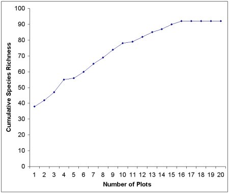
Figure 3. An example of a species accumulation curve. Sampling is adequate if the curve approaches an asymptote, which is the inflection point or where the line begins to become level. The asymptote is also the estimate of species richness.
The biologists that collected the data shown in Figure 3 appear to have sampled adequately because the curve approaches an asymptote, in other words, the curve levels off with increased sampling effort. The best estimate of species richness of this plant community is 92, shown by the point where the curve approaches the asymptote.
Activity 2: Species accumulation curves
Next you will create two species accumulation curves: one for the Bison-Absent watershed (data listed in the Activity 2a spreadsheet) and one for the Bison-Present watershed (data listed in the Activity 2b spreadsheet).
Directions
- The Activity 2a spreadsheet contains plant species composition data for the watershed without bison. The Activity 2b spreadsheet contains the plant species composition data for the watershed with bison. Each sheet has 20 subsets of data. The first subset contains the species present in the first plot, the second subset contains the total species present in the first and second plots combined, the third contains the species present in the first, second, and third plots combined, etc. With the data arranged this way, we can calculate the cumulative species richness as we add an additional plot one at a time. These are the data needed to create a species accumulation curve.
-
Calculate the species richness for each subset in the Activity 2a and 2b spreadsheets. The species richness values should be in row 59 of Activity 2a and in row 99 of Activity 2b in the cells with black borders. Refer to the instructions under
Before Beginning
if you need additional help. Here is where theNumSpec
function will really speed things up. -
Plot the cumulative species richness against sampling effort (number of plots). Note that at the right of all of the data subsets there are two columns labeled
Number of plots
andSpecies richness.
The first column contains the number of plots (1, 2, 3, …, 20). The second column will contain the species richness values you calculated in step 2.To get these values in column form from row 59, CTRL click on each value, and click Copy in the Edit menu. Move the cursor an empty column cell, click Paste Special in the Edit menu, mark Values and Transpose, then OK. Now you should have two columns of numbers: number of plots and a corresponding species richness value.
In order to create the graph:
- Highlight the column of species richness values. Do not highlight the column title.
- Click on the Chart Wizard icon in the tool bar.
- Under chart type, select Line. Several Chart sub-types are available. The default option is the one we want to use for this graph. Click Next.
- The next screen shows a Preview of your graph. If everything looks correct, click Next. If things are not correct, re-select the data you wish to graph.
-
The next screen allows you to add important information to your graph. Click the Titles tab. Add labels for both axes (x-axis should be
Number of plots
) and a title indicating the treatment. - Click the Legend tab. Because we have only a single line on our graph, we do not need a legend. Uncheck the Show legend box. Click Next.
- The last window asks if you wish to display the chart in a new worksheet or as an object in the current worksheet. Choose As an object and click Finish.
- If you wish to move your graph, use click and drag.
- Repeat steps a-h with Activity 2b. Recall that your species richness values should be in row 99.
Questions for Activity 2
Question 4. Were an adequate number of samples taken? Provide evidence to support your claim.
Question 5. Can we estimate species richness from these species accumulation curves? Why or why not? Support your answer with the data and figures you've just examined.
Question 6. Using the new information obtained from the species accumulation curves, how would you answer our original question: What is the effect of bison grazing on plant species richness?
Conclusions: Species richness and sample size
Species richness is intuitively easy to interpret and is often a central concern of conservationists. While it does not necessarily give the whole picture of diversity (remember, diversity includes both richness and evenness!) it can be very useful in many situations.
Species accumulation curves are only one of the tools available to biologists to estimate species richness. In the mid 1990's, significant advances occurred in what are called nonparametric estimators of species richness that use mathematical formulae rather than relying on interpretation of plots to calculate species richness. For instance, Magurran (2004) discusses several of these estimators and their appropriate use for different applications. There are specific computer programs that biologists use to calculate these estimates. Although we will not explore them further in this exercise, such estimators are well described in Magurran (2004).
Question 7. When might species richness be the primary diversity measure of interest? What cautions do biologists need to keep in mind when interpreting species richness?
Concept 3: Exploring diversity
Recall that measuring species diversity is based upon two ideas: species richness and species evenness. Now that we know how to measure species richness and how to interpret these measures, we will include evenness to our diversity measures. Although many indices have been developed that incorporate both species richness and species evenness into a single measure of diversity, we will explore two of the most common, the Shannon Index and the Simpson Index. But first we need to understand how to measure evenness and relative abundance.
Evenness and relative abundance
Refer back to Table 2, and recall that evenness measures how equally abundant the species in a community are. For example, a community with nearly equal abundances of all species, such as in Site 2 of Table 2, would be considered extremely even. Therefore, in order to measure evenness, we need to know the abundance of each species present in the community and how that abundance compares with all the other species in the community. The number of individuals is an obvious and common measure of abundance and should be used when an individual is readily distinguishable, such as with birds, mammals, insects, trees, and annual plants. Several organisms, such as clonal plants, fungi, and bacteria, can pose difficulties in discerning where one individual ends and another begins. In such cases, biomass, frequency, cover, and cover class are other measures of abundance. To understand how abundant a species is in a given community, we need to compare it to the rest of the community, and we can do this by using relative abundance. To calculate a relative abundance value for a given species, we take the abundance of the given species and divide it by the total abundance of all species in the community of interest. In our case we will use frequency as our abundance measure to address the question: what is the effect of bison grazing on plant diversity in tallgrass prairie?
Frequency is defined as the proportion of total sample plots in which that species was found. For instance, if Lespedeza capitata (round headed bush clover) were found in one-fourth of the plots sampled, its frequency would measure 0.25. The Excel spreadsheet for Activity 3 already contains the frequency values for each species found in each treatment.
To calculate relative frequency for our Konza data, we will take the frequency of each species and divide that by the sum of the frequencies for all of the species in the community. Using the example from above to calculate relative frequency for L. capitata, we would take 0.25/(sum of the frequencies calculated for all species in the community). We will calculate the relative frequencies in this way in our Excel spreadsheet.
Shannon Diversity Index
The Shannon Index uses relative abundance data (in our case, we will use relative frequency) to incorporate species evenness and species richness into a single measure of diversity, represented by H'. The Shannon Diversity Index typically falls between 1.5 and 4.0, with lower values indicating lower diversity, and higher values indicating higher diversity.
Here is the equation for the Shannon Index:
H' = -Σ pi ln(pi)
We'll build this equation up, starting with the term on the far right:
- pi is the relative abundance of each species i, as explained above.
- ln(pi) is the natural logarithm of the relative abundance.
- pi ln (pi) is the relative abundance of species i, multiplied by the natural logarithm of the relative abundance (pi). We calculate this product for every species in the community.
- Σ pi ln (pi) is the sum of the pi ln (pi) products that we calculated for every species in the community.
- -Σ pi ln(pi) is the negative sign of the sum that we calculate. This is necessary because taking the natural log gives us a negative number. Positive numbers are much easier to interpret. This gives us H', the Shannon Diversity Index.
One could easily use a calculator or spreadsheet to figure each of these steps. But we are going to take advantage of a program that has already been written to do these calculations in Excel in one step. Mathematically it is a measure of the average degree of uncertainty
in predicting the identity (species) of an individual drawn randomly from the community.
Activity 3: Shannon Diversity Index
Directions
- Go to the Activity 3 spreadsheet in the Konza Diversity Exercise Excel workbook. These data were taken from the watershed with bison present. Notice that there are four data subsets within this spreadsheet. Each subset contains the species present in that watershed and their abundance measured by frequency.
- Calculate the species richness for each subset using the Numspec function (see Activity 1 for review).
-
Calculate the Shannon Index for the first data subset, N = 4.
- Select an empty cell below the frequency data for the first subset.
- Under the Insert menu, select Function.
- In the Function category box, select User Defined.
- In the Function name box, select Shannon.
- Click OK.
- Select the cells containing all of the frequency data in the first data subset.
- Click OK and the Shannon Diversity Index value should now be displayed in the cell. The answer for data subset 1 should be approximately 3.705.
- Repeat steps a-g for all four data subsets.
-
Complete the first three columns of Table 5 with your results (the last column, D, will be filled in later). Again, give the table a descriptive title.
Table 5. S N H' D S = species richness, N = sample size, H' = Shannon Index, D = Simpson Index
Simpson Index
A potential drawback of the Shannon Diversity Index is that it is very sensitive to species richness. That is, if an additional species is added, the Shannon Index rises disproportionately, especially if the new species is not abundant. A different measure, the Simpson Diversity Index, is heavily weighted by abundances of the most common species, and produces a measure that is less sensitive to species richness. For instance, we would likely consider a community truly more diverse if it had equal abundances of 25 species, than if it had one very dominant species, and 24 extremely rare species. The Simpson Index, represented as D, gives more weight to the relative abundance of species in a community in that it is based on the probability that two individuals drawn from an infinitely large community are the same species. This is the equation:
D = Σ pi2
- pi is the relative abundance of species i (and this is then squared).
- Σ pi2 is the sum of the values that we calculated for every species in the community.
As D increases, diversity decreases, which is rather counter-intuitive. For the value to be more intuitive, the Simpson Index is usually expressed as 1-D or 1/D, so that the value actually rises as the community becomes more diverse. We can use the Excel spreadsheet to calculate the Simpson Index in a few easy steps. Although the diversity plug-in we installed does calculate the Simpson Index, it does so using a different measure of abundance than we are using, so we will program the formula ourselves in Excel to take into account the measure of abundance taken at Konza Prairie, that is, frequency.
Activity 3: Simpson Diversity Index
Directions
To calculate the Simpson Index for each data set:
- Open the Activity 3 spreadsheet again to calculate the Simpson Index. Place your cursor in the cell next to the first frequency data point in the empty column of first data set (cell D5). This will become your formula cell.
- Type = (
- Click on the first frequency data point. You will see that the reference for this cell shows up in the formula cell so that it should now read = (C5
- Within the formula cell, type / (sum(
- Using your cursor, select the entire column of frequency values.
- Your formula should now look like this: = (C5 / (sum(C5:C49
- Add $ as shown here: sum($C$5:$C$49
- Type )))^2 and hit enter
- Your formula should read: =(C5/(SUM($C$5:$C$49)))^2 and the correct result is 4.5E-05.
- Fill this formula all the way down this column until you reach row 49. One way to do this is to highlight the entire column between row 5 and 49. Under the Edit menu, select Fill and then Down.
- Place your cursor in the first empty cell under the column of numbers you just created (cell D50).
- Type the following formula: = 1 – sum(
- Select all of the data just above this cell (cells D5:D49)
- Within the formula cell, type ) and hit Enter. The entire formula should read = 1-sum(D5:D49)
- The value in this cell is the Simpson Index and should be approximately 0.97 for the first data subset.
- Repeat steps 1 – 15 for the remaining 3 data subsets on the worksheet.
Complete the last column in Table 5 with your results.
Question 8. How does species richness affect the Shannon and Simpson Diversity Indices? Given what you already know about how sample size affects the calculation of species richness, how do you think sample size would affect the Shannon Index? The Simpson Index?
Activity 3: Comparison
Now that we know something about how to calculate diversity indices as well as a little bit about their pitfalls, let us return again to our original question: How does the presence of bison affect plant species diversity?
Calculate the Simpson Index using data provided in the Comparison spreadsheet. Refer to step 2 above for directions.
Question 9. What is the effect of grazing on tallgrass prairie diversity? Compare your answer with the conclusions you drew based upon species richness alone. Why are your conclusions similar or different?
Question 10. When might a diversity index (instead of just species richness) be the primary diversity measure of interest? Why?
Conclusions: Diversity indices
Despite the fact that several studies have shown that the Simpson Diversity Index performs much better, the Shannon Diversity Index is the most widely used. In fact, Magurran (2004) states, The Simpson's index is one of the most meaningful and robust diversity measures available.
Further, she points out the serious shortcomings of the Shannon Index, including its sensitivity to species richness, and thus, sample size. One benefit to using the Shannon index is that it allows a researcher to compare their results to past studies. While the Simpson Diversity Index is often a better choice, it is not a panacea. All diversity indices, including the Simpson Diversity Index and the Shannon Diversity Index, are based on some weighing of relative abundance and species richness, but each index weighs these measures differently. For this reason, scientists often calculate several indices for their data, or choose one index carefully based on what they know about their study system and the assumptions made by a given index.
[ TOP ]
Part 3: Assumptions and Conclusions
In her classic book on measuring biodiversity, Dr. Anne Magurran (2004) lists three assumptions of biodiversity measurement.
- All species are equal. In other words, rare or endangered species are no more important than the most common species in the community.
- All individuals are equal. In other words, the largest redwood in the forest is given equal weight with the tiniest redwood seedling.
- Species abundances must be measured appropriately. In addition, it is important to use the same abundance measure at sites or times that you wish to compare.
Question 11. Why is it important to understand the assumptions behind biodiversity measurements? What information would you need to evaluate whether or not the assumptions had been met or are appropriate?
Assumptions Specific to Shannon and Simpson
In addition to the general assumptions listed above, the Shannon and Simpson Indices have a few more assumptions associated with them.
Shannon Index
Assumption 1: Individuals are randomly sampled from an infinitely large community.
Assumption 2: All species are represented in your data set. In other words, if a species is present in a community, you sampled it. If you didn’t encounter the species, it doesn’t occur in the community.
Simpson Index
Assumption 1: Individuals are randomly sampled from an infinitely large community.
There is a version of the Simpson Index that does not require Assumption 1. If the researcher feels that this assumption cannot be met, the modified Simpson Index can be used. As you can imagine, the modified Simpson Index is a bit more computationally complex, which is why we will not go over it for this exercise. There is no equivalent correction for the Shannon Index.
Question 12. Recall that the Shannon Index has been widely used. How often do you think the assumptions for using the Shannon Index have been met? The Simpson Index?
Conclusions
By comparing just these two watersheds (Bison-Present and Bison-Absent), our data indicate that bison grazing may increase plant diversity. Long-term research at Konza Prairie substantiates this indication. Statistical analysis conducted on data from many replicate watersheds of these treatments over time has shown that bison have two main effects on the tallgrass prairie plant community that serve to increase plant diversity. First, bison create a more heterogeneous environment by wallowing, by creating grazing lawns, and by excreting wastes, opening more sites for different types of plants to colonize and grow, increasing species richness (Hartnett et al. 1996). Second, bison prefer to graze on the major dominant grasses, such as A. gerardii (big bluestem). By grazing down the dominants, bison create a competitive release of the sub-dominant vegetation allowing plants to flourish that may otherwise be out-competed by big bluestem if the bison were not present, often leading to increased species evenness (Knapp et al. 1999).
We have practiced two main tools that biologists use to quantify species diversity:
- species richness or simply counting the number of species present in an area
- species diversity that incorporate species richness with information about the abundance of each species in the community.
In both cases, we have explored the influence of sample size on the measurement of species diversity.
Conserving biodiversity is an important goal, but through the activities presented here, we have seen that it is not always straightforward to measure what we wish to conserve. Applying the appropriate tools to measure biodiversity is an important step toward our goal of conservation as well as understanding patterns of biodiversity loss in communities.
[ TOP ]