
VOLUME 4: Table of Contents
TEACHING ISSUES AND EXPERIMENTS IN ECOLOGY
Modeling has become an important tool in the study and management of ecological systems (e.g., Brennan and Withgott 2005). Sometimes it is not possible to manipulate an ecological system to test rival hypotheses in field tests. For example, costs and time constraints can limit large-scale experiments for testing community responses to an environmental disturbance. In contrast, models can help explore hypotheses quickly and rigorously, and can help to define research questions and identify data needs (e.g., see May 1973, and Levin 1974 for discussions about theoretical predator-prey models). While modeling is widely considered by ecologists to be an important component of ecological education, most ecology students have the misconception that ecological models (particularly those dealing with ecosystems and communities) are always extremely complex and filled with mathematical equations (a quantitative approach). On the contrary, a complex ecological system can be simply yet formally described with a set of 'boxes and arrows' (a qualitative approach).
Models are simplifications of real systems. They can be used as tools to better understand a system and to make predictions of what will happen to all of the system components following a disturbance or a change in any one of them. The human brain cannot keep track of an array of complex interactions all at one time, but it can easily understand individual interactions one at a time. By adding components to a model one by one, we develop an ability to consider the whole system together, not just one interaction at a time. Models are hypotheses. They are proposed representations of how a system is structured, which can be rejected in light of contradictory evidence. No model is a 'perfect' representation of the system because, as mentioned above, all models are simplifications. In working together to build your models using the methods described in the next section, you will generate new hypotheses about interactions occurring within the ecosystem that provide a better understanding of the complexities of the ecosystem as a whole.
Signed digraphs. Qualitative models are typically drawn as familiar and intuitive "signed digraphs" (diagrams that describe the relationship of community species based on sign of interactions, with positive effects denoted by an arrow and negative effects denoted by a line terminating in a filled circle) consisting of ecological 'components' (in boxes or circles) and positive or negative 'links' (Jeffries 1974, was one of the first to use of this term in ecology literature). A component is any variable part of an ecosystem. A population of a given species, the amount of nitrogen held in the soil, and the temperature of the water in a stream could all be identified as ecosystem components. Links are symbols that represent interactions occurring between components. These can be used to show a flow of materials or energy between components, or can be used to indicate a causal effect of one component on another. The term 'system' refers to any combination of two or more components that have some form of interaction between them.
Interactions between populations of different species in a community can be classified with combinations of the three symbols {-,0,+}. In general, there are 5 types of interactions: commensalism (+/0) (Fig. 1a), amensalism (-/0) (Fig. 1b), mutualism (+/+) (Fig. 1c), predator-prey (+/-) (Fig. 1d), and interference (-/-) (Fig. 1e).
 1a) Component 2 has a positive effect on component 1 without any effect on itself. For example, if the sun is component 1 and plants are component 2, plant growth and reproduction are enhanced with increased exposure to solar radiation, but this has no effect on the sun. This relationship is not a feedback loop because there is no return signal (input) to component 1.
 1b) Component 1 has a negative effect on component 2 without any effect on itself. For example, non-breeding adult Nazca boobies (component 1) nest near the sites where blue-footed boobies (component 2) nest. Adult Nazca boobies will attack blue-footed boobies nests and injure nestlings, which prevents them from fledging. This interaction does not result in any benefits (such as effects on fecundity and survival) for the adult Nazca boobies. This relationship does not constitute a feedback loop because there is no return signal (input) to component 1.
 1c) Two components positively affect each other. If each component is biological, this relationship is referred to as a 'mutualism.' If component 1 represents flowering plants and component 2 bees, flowers provide food while the bees help the plants to reproduce. This relationship is a positive feedback loop since the signs of the input and output are the same (here they are both positive).
 1d) Component 2 has a positive effect on component 1, but component 1 has a negative effect on component 2. This relationship between a predator and its prey could be represented by this digraph. As the predators (component 1) increase in numbers, they deplete the prey (component 2), which in turn has a decreasing effect back to the predators. Likewise, as the predators decrease in numbers, the prey benefit from reduced predation and this has an increasing effect on the predators as a result of increased food resources. This is a negative feedback loop because, for either component, the input is opposite in sign to the output.
 1e) Two components negatively affect each other. Two species in competition for the same resource can lead to this type of interference. Note that, in effect, this relationship constitutes a net positive feedback loop because the signs of the input and output are the same (they are both negative). The net effect is positive feedback since, as explored by May 1973, this interaction will result in instability — unless it is mediated by regulatory processes stemming from self-regulation or from interactions with other components.
Feedback loops. A feedback loop occurs when a signal leaves one component (output) and returns to the original component (input) after passing through one or more other components in the system. If the signs of the output and input signals are the same (either both positive or both negative), then it is a positive feedback loop. This includes competition (-/-) and as May (1973 & 1974) pointed out, neither mutualisms nor competition lead to stability because of this NET positive feedback qualitative relation. May (1973) also neatly observed that this may appear to be counter-intuitive. If the signs of the output and input signals are opposite, then it is a negative feedback loop. Thus, Figure 1d depicts a negative feedback loop, since the link from predator to prey is negative while the link returning to the predator from the prey is positive. An increase in predators results in a decrease in prey, the decrease in prey then causes a decrease in predators, the decrease in predators then causes an increase in prey, etc. In general, through this moderating effect, negative feedback loops promote stability in systems. Figures 1c and 1e are both positive feedback loops, because output and input signals have the same sign, and these types of interactions tend to be destabilizing. Figures 1a and 1b do not constitute feedback loops since no signals return to the original components.
Figure 2. Illustration of a self effect (self-limiting) loop symbol.
Self limiting, self regulating, or density dependent components, such as plants, should include a symbol indicating a "self effect" loop, as shown in figure 2. This is required because in nearly all situations the plants are competing for limiting water or nutrients in the soil; any nutrients that go to one individual are thus denied to the others in its species or component type.
Any circuit of interactions produces feedback, as shown in figure 3. As mentioned above, a feedback is negative when the product of each of the signs in the loop is negative and when there is an odd number of links. A negative feedback loop is a very important concept in producing stability in a system. A negative feedback loop returns a signal to a component that is opposite in sign to the signal that left the component, thereby stabilizing the system. The most familiar example of a negative feedback system is the thermostat. If the room cools down below a set temperature, the thermostat responds by turning on the furnace that will heat up the room. When the room temperature increases to a level above the temperature set on the thermostat, the thermostat will shut down the furnace.
Figure 3. Three feedback loops of a three species community
Figure 4 illustrates how these digraphs can be linked to generate a more complex ecosystem model. In a model containing more than two components, both 'direct effects' and 'indirect effects' can result from a change in a given component. Indirect effects are those that occur as a result of a change in a component that is not immediately connected to the original component (two or more links separate the two components). According to the model shown in figure 4, if root-feeding click beetle populations increase, the amount of root mass should decrease. This is a direct effect because there is a single link separating these two components. As a result of this decrease in root biomass, the amount of its mycorrhiza, the root-symbiotic fungus, present in the soil may also decrease. The decline in root-symbiotic fungi occurring as a result of adding click beetles to the system is an indirect effect because the fungi and beetle components are separated by more than one link.

Figure 4. A sample model of a soil ecosystem using the signed digraph convention
Ecologists use this type of model as the basis for 'loop analysis.' This type of analysis can provide indications of the stability of a given system either as it currently exists or, often, as it might exist following a change in the current system due to some type of management practice or disturbance (e.g., deer populations if foresters cut half of the oak trees or fish populations if hunters are allowed to shoot ducks, etc.). Feedback loops, and the positive and negative links that constitute them, are analyzed at different levels to determine whether certain stability criteria are met. The analysis can then proceed to evaluate whether each of the various components will either increase (+), decrease (-), or remain unchanged (0) following a 'disturbance.' This analysis involves qualitative (+, -, 0) rather than quantitative (exact numerical) changes, and is referred to as qualitative analysis.
In loop analysis, instead of considering the effects of a parameter change (change the coefficients of a community matrix) on a system variable (the population density of a species in a community), the overall effect of an input (positive or negative) on one given component by another component is calculated. The overall effect is negative if the product of multiplying the signs of all the feedbacks results is a negative (-1). The overall effect is positive if the product is positive (+1). If the number of positive feedbacks equals the number of negative feedbacks, then there is no net effect of the change in one component upon another. The set of these effects for all pairs of components in the community is often referred to as the prediction matrix or matrix of the directions of change of the model components that can be used to predict the effect of an input on all community members. In Part 2, you will learn that mathematically the prediction matrix equals the adjoint of the community matrix.
Student Handout 1: Introduction to Qualitative Modeling (*.doc 48KB)
or (*.pdf 61KB)
Student Handout 2: Steps for Creating Qualitative Models (*.doc 29KB)
or (*.pdf 20KB)
Today you will travel to a field site in a local ecosystem, observe biotic and abiotic interactions among the organisms that live there, and, based on these interactions, create a qualitative ecosystem model using the symbolic signed digraph notation just presented.
While at the field site or immediately upon return, write down as many ecosystem components as you can based upon your observations during the field experience, information you have read, and our in-class discussions. You should generate a model that 1) hypothesizes how these components interact with each other and with the rest of your study ecosystem, and 2) communicates the extent of your knowledge about the ecosystem.
Modeling has become an important tool in the study and management of ecological systems. An ecological system or process often cannot be directly manipulated in a field test. Costs and time constraints can limit large-scale experiments for testing community responses to an environmental disturbance. In contrast, models can help explore hypotheses quickly and rigorously, help to define research questions, and identify data needs.
Please review the concepts in Student Handout 1 (*.doc 48KB) or (*.pdf 61KB) and review the information in the introduction above.
Here are the exact steps to follow for creating your qualitative ecosystem model (see Student Handout 2 [*.doc 29KB] or [*.pdf 20KB]). Work alone on this part:
It is useful at this point to pause and review the following aspects of qualitative modeling for a simple ecosystem containing only three biotic components. Consider the following simple model. Notice that feedback, direct effects, indirect effects, and descriptions of the key interactions are illustrated. The ability to easily identify indirect effects of perturbations is one of the main strengths of this type of qualitative model.
Figure 5. Example of a model with descriptions of each interaction.
Discussion question — Note the arrows denoting positive effects, and the one instance of negative feedback. Discuss the difference between direct and indirect effects. What are some examples of indirect effects in the figure?
Discussion question — Propose a potential human-caused impact, such as an invasive species, to this ecosystem and add it as a new component to the model. Add links connecting the new component to the other component(s) that would be directly affected. What are all possible indirect effects (effects on components two or more steps away from the new component) that may occur as the original perturbation spreads through the components in the system?
Choose a partner to work with for the next steps. For each question, first think about and write down your ideas, then each take a turn to describe your response to the other. If during the discussion you get additional ideas, write them down too.
The qualitative analysis described in Part 1 serves as an excellent exercise to show students a way to approach a complex system, to help students to begin thinking about complexity and indirect effects, and even to allow students to generate hypotheses about what could happen to an ecosystem following a change in one or more of its components. However, if we are interested in making detailed predictions, this informal type of qualitative analysis may not be able to account for the ultimate effects of a disturbance on a system of interest. This is because a complex, interacting system can behave in unexpected ways that are not simply the "sum of its parts." These "emergent properties" of systems can only be captured with more detailed analyses.
Part 2 presents steps for constructing qualitative models and loop analyses using a web-based computer application. We have converted the procedures of loop analysis to software containing well-known matrix algebra functions, which removes tedious hand calculations and minimizes errors. We also provide a graphical program in POWERPLAY that is especially useful for drawing a large community system with many variables and reducing transcription errors when the signed digraph converts to a matrix.
The desktop POWERPLAY is available for free from the Ecological Society of America's Ecological Archives (http://esapubs.org/Archive/ecol/E083/022/suppl-1.htm), from the POWERPLAY downloads page (http://www.ent.orst.edu/loop/download.aspx), or from the TIEE Downloads page for this experiment (downloads.html).
POWERPLAY is a Java-based program providing a friendly graphical interface so that users can easily develop an ecological community model. POWERPLAY has three visible parts. There is a menu at the top, a workspace (the large blank area in the window), and the toolbar. The menu provides a way to change optional settings and to access files and other features of POWERPLAY. The graphical representation of the digraph appears in the workspace and can be modified using the mouse and the tools. The toolbar provides alternative ways to manipulate the digraph.
Once installed, there are several command buttons on the POWERPLAY web page.
The user can click on these buttons to accomplish the following technical tasks:
In this section, we use real ecological research data to demonstrate loop analysis of an aquatic system in which an invasive species has been introduced. This example is provided by Michael Chi-Chun Liu, a Fisheries and Wildlife graduate student from Oregon State University. We will use the prediction matrix from loop analysis to suggest several management scenarios in which the reduction of the invasive species is predicted.
The New Zealand mud snail, Potamopyrgus antipodarum, was first discovered in the United States in the mid-Snake River, Idaho in the 1980's. It is a parthenogenetic (a reproduction behavior where the growth and development of an embryo or seed occurs without fertilization by a male) livebearer with high reproductive potential, and is now a rapidly spreading problem throughout the western USA. It has become established in rivers in 10 western states and three national parks. Because of its reproductive potential, the mud snail has reached densities of 100,000/m2 in some habitats. This rapidly growing invasion has created problems for fisheries and aquatic ecosystems in the western USA, where there is concern about the potential harmful effects on native species.
Possible Ecosystem Models: Liu developed a series of models using five different sets of predictions about how either fertilization or the reduction of nutritional input would decrease the population of the New Zealand mud snail in the lower area of the Columbia River. These models were based on published literature and expert opinion. Using the prediction matrix of loop analysis, we will concentrate on the potential of these variables to reduce the population of mud snails in the lower area of the Columbia River. Many of these potential impacts can only be assessed through an analysis of community interactions. These models will be compared to information on trophic relationships generated from the previous study. Experiments and field studies will then determine which of these projected models is the most suitable for testing our ecological hypotheses.
 (6A) Model 1 is the grazing model. Algae is the sole source of primary production in this system, and is thus the only variable for which New Zealand mud snails and aquatic insects compete. The top predator, smolt (a fish), has a self-regulated loop and feeds on aquatic insects rather than the New Zealand mud snails. Model 1 is a general model that can be used to represent any aquatic system encountering an invasive species.
 (6B) Models 2 and 3 are based on New Zealand mud snails and native aquatic insects having different food preferences. In Model 2, the two grazers feed on different species of algae. In Model 3, aquatic insects only feed on one group of algae, but the New Zealand mud snails graze on both groups of algae.
 (6C) Model 4 is the grazing/space competition model. In this model, New Zealand mud snails not only graze on the algae, but because the alga grows densely, covering the substrate, the mud snails also compete with the algae for limited space.
 (6D) Model 5 introduces the idea of functional groups. In this model, smolt benefit mud snails by feeding on both grazer and collector aquatic insects; New Zealand mud snails compete with grazers for food resources (algae) and with collectors for space.
Out of the five models, Model 1 represents a simple aquatic system, a food chain plus an invasive species. In contrast, Model 5 represents a very complex and realistic aquatic system. We will use Model 1 to illustrate how POWERPLAY can create a digraph for a community system and the loop analysis to analyze the system. We will use both Model 1 and Model 5 to discuss the predicted outcome, i.e., the direction of the impact on all species when a positive/negative effect is added to a particular species. The management goal is to determine how the population of New Zealand mud snails can be reduced with the least impact on the native species.
Using POWERPLAY: To create a community system model in POWERPLAY, we click on the node
tool (![]() ) from the tool bar, and then click in the workspace where we want
nodes to appear. The default names of nodes are a series of sequential numbers. When we
right-click on a node, a small dialog box pops up which allows us to edit, delete, or rename the node. If you want to change
the names of the node to something else just right click on it to bring up the editor menu and then change the name and
press enter.
) from the tool bar, and then click in the workspace where we want
nodes to appear. The default names of nodes are a series of sequential numbers. When we
right-click on a node, a small dialog box pops up which allows us to edit, delete, or rename the node. If you want to change
the names of the node to something else just right click on it to bring up the editor menu and then change the name and
press enter.
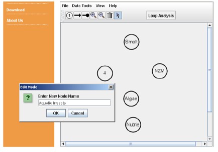
Figure 7. Building qualitative ecosystem models in POWERPLAY.
After the nodes have been created, we can make the effect arrows. To create the arrows, from the tool bar
(click either ![]() or
or ![]() ),
on the first node in the relationship and drag the pointer to the target node. Note that the first node clicked on is the
source of the effect (either positive [blue] or negative [magenta]) and the second is the affected node. We can place a
"self-effect" on a node by double clicking on the target node with the appropriate effect tool. The weighted default
interactions between two nodes are (-1, +1, 0), indicating a negative effect, positive effect, or no effect. If there is
no connection between two nodes, the weight is 0. If there is a connection (either positive or negative), the weights of
the effects can be changed as needed by right-clicking on the connection between two nodes to open the pop up menu, change
the value, and pressing return. The effect will change to the appropriate type and color if the sign changes but, other
than the effect type, there will be no outward display of the weight. Click on the Show Matrix View found in the Data
Tools menu to pop up a dialog box that displays the contents of the workspace in matrix form.
),
on the first node in the relationship and drag the pointer to the target node. Note that the first node clicked on is the
source of the effect (either positive [blue] or negative [magenta]) and the second is the affected node. We can place a
"self-effect" on a node by double clicking on the target node with the appropriate effect tool. The weighted default
interactions between two nodes are (-1, +1, 0), indicating a negative effect, positive effect, or no effect. If there is
no connection between two nodes, the weight is 0. If there is a connection (either positive or negative), the weights of
the effects can be changed as needed by right-clicking on the connection between two nodes to open the pop up menu, change
the value, and pressing return. The effect will change to the appropriate type and color if the sign changes but, other
than the effect type, there will be no outward display of the weight. Click on the Show Matrix View found in the Data
Tools menu to pop up a dialog box that displays the contents of the workspace in matrix form.
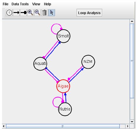
Figure 8. POWERPLAY example of mud snail community with effect arrows inserted.
Loop Analysis: The basic structure of the digraph is placed in the workspace. It is now time to do the loop analysis by clicking the "Loop Analysis" button which causes the loop analysis web page to appear. This page provides several buttons and a text box for entering a community matrix using a text string reflecting the structure of community system. The format follows the Maple syntax for matrix algebra format (Dambacher et al. 2002). If the user uses POWERPLAY to create a digraph of community system, the text string of the community matrix is automatically generated. If the user does not want to use POWERPLAY to create a digraph and a matrix, the user can enter the matrix to the text box. The matrix syntax is based on the Maple syntax for matrix algebra (Dambacher et al. 2002). For those who are interested in the procedure to solve the ordinary differential equations, Dambacher et al.s program can run both qualitative and symbolic analysis of the community matrix. The program is available at the Ecological Society of America's Electronic Data Archive. The user can still use POWERPLAY to create a digraph and the text string of the community matrix. The text can be copied and pasted to Dambacher et al.s Maple program, which will save the time required to enter the matrix manually.
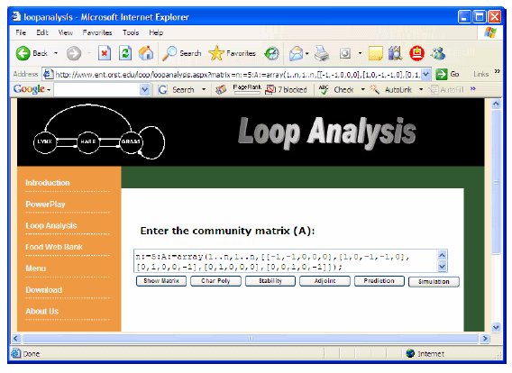
Figure 9. Text string of community matrix of mud snail example in POWERPLAY.
The "Show Matrix" button is used to check the matrix form and show a generic digraph based upon the input text string.
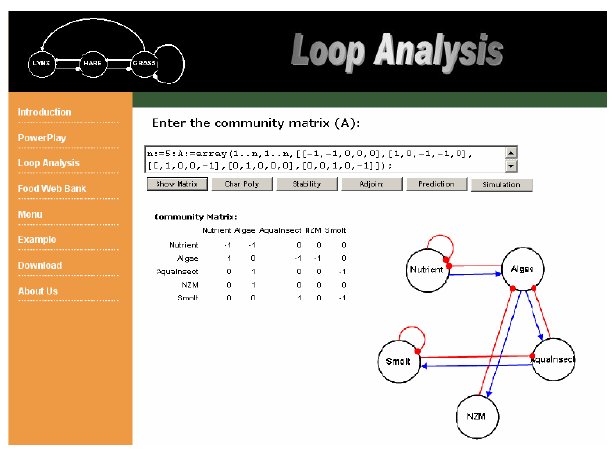
Figure 10. Example of generic digraph based upon input in POWERPLAY.
The "Char Poly" button is used to calculate the coefficients of the characteristic equation, which represents different levels of feedback. System stability requirements are derived from the coefficients (cn) of the characteristic equation.
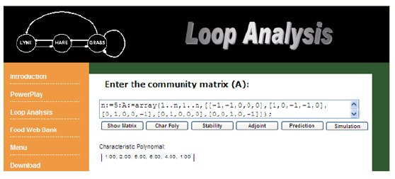
Figure 11. Example of Char Poly calculation in POWERPLAY.
The "Stability" button is used to test the system stability that is based on two criteria:
This is calculated from the Hurwitz matrix which is constructed from the coefficients of the characteristic polynomial function.
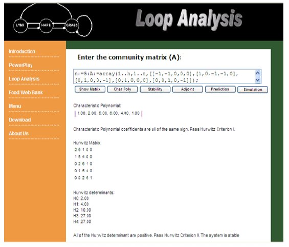
Figure 12. Example of community stability calculation in POWERPLAY.
The "adjoint" button is used to display the adjoint of the community matrix, the absolute feedback matrix, and the weighted prediction matrix. The adjoint of the community matrix computes the sensitivity of any variable to the change of system parameters. Mathematically, the elements of the adjoint matrix are the cofactors of the transposed matrix. Thus, a change in the population abundance of a species is determined by the net effect of complementary feedback loops, i.e., the subsystems not in the direct path of these species. The adjoint of the community matrix can be viewed as a prediction that provides an estimate of the change in equilibrium abundance of each system member resulting from a positive/negative impact. Positive input effect to the adjoint matrix is read down to a column that contains the responses of all species in the system. A positive number represents a positive response, a zero represents no response, and a negative number represents a negative response. Because the adjoint is the sum of positive and negative loops, we do not know the numbers of positive and negative loops in the subsystem. An absolute feedback matrix (using the same calculating method as the adjoint except for taking absolute value for all elements in the calculation) can detail the total number of complementary feedback loops involved in each community response. Lastly, a weighted prediction matrix scales the response of adjoint and allows for the reliability of each predication.
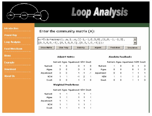
Figure 13. Example of prediction output using POWERPLAY.
The "Prediction" button displays an interactive graph for each the adjoint matrix. The user can click the column header of each species to mimic a positive impact to the species of column header and display the response of all community species to the positive input.
The "simulation" button conducts a simulation using randomly generated quantitative matrices to evaluate the probability that the system is stable quantitatively. The stability test is based on the signed digraph, in which the relationships between species are (+1, -1, 0). The qualitative stability offers no insight into the stable structure of quantitative domain of the system. For example, a signed digraph has an overall negative feedback with two negative loops (-2) and one positive loop (+1). However if we have the measure of interaction strengths between species, the values of two negative loops may be -0.2 and -0.3, and the value of positive loop may be 0.6. In this case the strength of overall feedback is 0.1 and then we will obtain a positive overall feedback. In order to know the probability that the system is also stable in a quantitatively specified matrix, 5000 quantitative matrices are constructed based on the unchanged sign structure of the system. Non-zero elements of each matrix are quantitatively specified with a pseudorandom number generator that assigns interaction strength but not a sign from a uniform distribution between 0.01-1.0. The stability of each quantitatively specified matrix is then examined in terms of stability criteria (Hurwitz criterion I: Characteristic polynomial coefficients are all the same sign and Hurwitz criterion II).
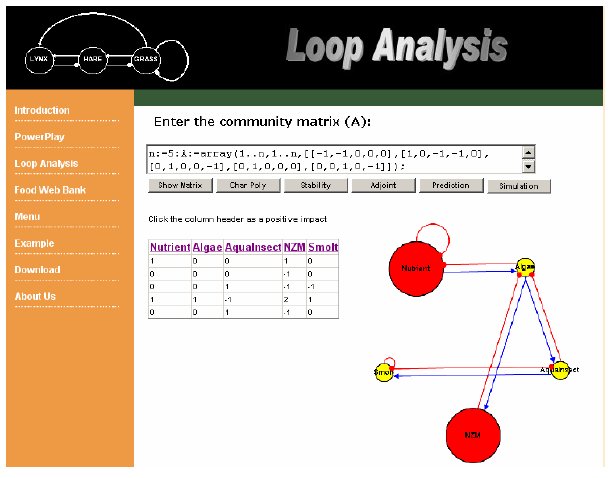
Figure 14. Example of graphic presentation of press experiment to adjoint matrix using POWERPLAY.
A bigger red circle represents a positive effect on the species, a smaller yellow circle represents a negative effect, and a white circle with the original size represents no effect.
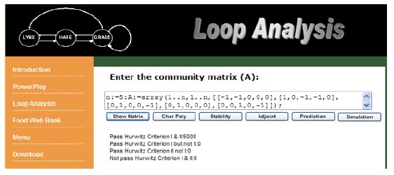
Figure 15. Example of simulation output using using POWERPLAY.
In the New Zealand Mud snails Model 1, when the snail continuously invades the aquatic system (we can consider that the invasion is a positive input to the New Zealand Mud snails), the impact will dramatically affect the native populations, decreasing algae, aquatic insects, and smolts. However, if the nutrient input can be reduced, e.g., by removing debris from streams, the population of New Zealand mud snails will decline and cause no negative impact on the native populations.
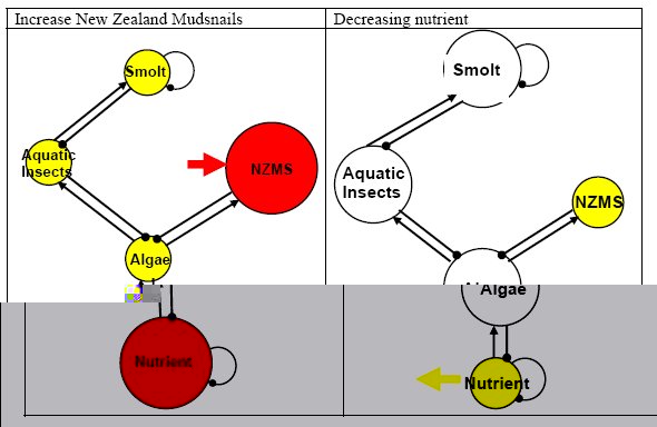
Figure 16. Scenario for New Zealand mud snail in decreased nutrient conditions in POWERPLAY.
For the New Zealand mud snail in Model 5, as we have seen in Model 1, continual addition of the snails will have a negative effect on all the native species. If the management goal is to prevent reduction of the smolt population, we can have several solutions based upon a "press experiment" (a permanent change on a system variable via increasing input or decreasing output, e.g., increasing the birth rate or decreasing the death rate) on the prediction matrix. We need to decrease the suitable space for the mud snails by adding large rocks along the shoreline. Alternatively, we can stock grazing or collecting aquatic insects in other ponds and continuously add them into the system to have a positive input effect on the grazing or collecting aquatic insects, which will press, or decrease, the population of the mud snails. However, if our management goal is to have the snail population decline and minimize the impact to the native species, we can remove the fish stock to another non-infested stream. This will result in a negative effect to the smolt population, which brings a negative effect on the New Zealand Mud snails, but generates positive effects on both grazing and collecting aquatic insects.
Students should keep in mind: the loop analysis alone can not be used to select the most accurate model when there are several models for the same ecological question. However, the prediction using the loop analysis technique can be applied to natural resource management to increase the required species or decrease the invasion species. Based on the simple and quick press experiment on the prediction matrix, ecologists can generate testable hypotheses for conducting experiments and field studies that will then determine which of these model structures is the most accurate.
Figure 17. Example of how to determine which model is more accurate using POWERPLAY.
For discussion:
In this part of the activity, you will create a digraph for a community system, use loop analysis to analyze the system, and show the direction of the effect of all species when a negative/positive effect is added to a particular species. We will run through the process first using the well-studied example of vegetation, hare, and lynx in order to study the relationships among these three species. Then, steps will be provided to generate models and hypotheses for your own research study.
Figure 18. Vegetation, hare, predator model showing negative feedback.
Prediction of system response — Use the "Adjoint" and "Prediction" buttons to create a prediction matrix and an impact diagraph which examine the response of the system to the impact of a particular species (the response of the vegetation, hare, lynx system to a permanently increased production of vegetation). An example of this calculation is provided below.
Example: The density-dependent effect represented in the above model for vegetation represents self regulation and is also depicted for predators, which have other important sources of prey in this model. Using the prediction matrix calculated by POWERPLAY for deriving effect of input, a positive response of vegetation to fertilization will cause a positive response on hares and predators.
Community matrix (Model I) = 
Prediction matrix (Model I) = 
Example: The density-dependent effect represented in the above model for vegetation represents self regulation and is also depicted for predators, which have other important sources of prey in this model. Using the prediction matrix calculated by POWERPLAY for deriving effect of input, a positive response of vegetation to fertilization is seen to cause a positive response on hares and predators.
Community matrix (figure 18) =
Prediction matrix (figure 18) =
However, Krebs et al. (1995) observed no response of hares to plant fertilization in contradiction to a positive response predicted in the example above. Dambacher et al. (1999) suggested a bottom-up commensal link between plants and predators, representing the likely benefit that plant cover provides to predators (figure 19).

Figure 19. Vegetation, hare, predator model with density dependent effects.
Community matrix (figure 19) = 
Prediction matrix (figure 19) = 
Predicted responses from figure 19 imply the existence of a hypothesized direct link between vegetation and predators. This link would neutralize any net benefit from a postulated fertilization experiment being passed on to hares. The zero net benefit may be translated by increasing vegetation, which in turn increases the birth rate of hares, but the increased birth rate of hares will be balanced by an increased death rate in hares due to predation by lynx. If figure 19 is correct and accurately represents an ecological community, what we can learn from the predication matrix is that increasing the vegetation abundance will not affect the hare population. In order to increase the hare population, a positive input on hares is required (see column 2 of the prediction matrix). This can be an increase in birth rates or a decrease in death rates of hares.
Questions for Discussion:
Here are the basic steps:
Choose a partner to work with for the next steps. For each question, first think about and write down your ideas, then each take a turn to describe your response to the other. If, during the discussion, you get additional ideas, write them down too.
Go to a computer and load your revised model into POWERPLAY.
Loop analysis can help ecologists to understand the community system and the relationships among species, by drawing a digraph, and to generate testable hypotheses by using press experiments (a permanent change on a system variable via increasing input or decreasing output, e.g., increasing the birth rate or decreasing the death rate) on the prediction matrix. Follow the illustration in figure 17 to analyze Models 2, 3, and 4 and answer the following question.
Models 2 and 3 are different only in the foraging behavior of the New Zealand mud snails. In Model 2, the New Zealand mud snails are seen as a specialist, feeding on only Algae 1. In Model 3, the New Zealand mud snails are seen as a generalist, feeding on both Algae 1 and 2. What can you predict to be the difference between these two systems if nutrient input to the system is reduced?
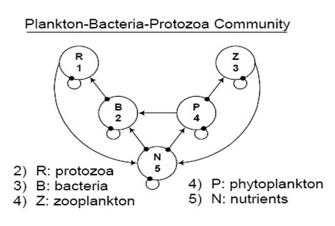
Figure 20. Plankton, Bacteria, Protozoa Community Digraph.
We often use a qualitative solution so that we can judge what changes of species interactions will affect the system stability. We can use matrix algebra tools to analyze the systems stability without knowing the precise value of all the parameters. We can continue to use our simple 3-species food chain model of a self-regulated plant (= 1), its herbivore (= 2) the snowshoe hare, and a specialized predator (= 3) the lynx, to understand the system feedback.
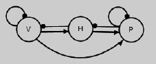
Figure 21. Vegetation, hare, predator model showing system feedback.
Ask students to do the same with their own models.
In the vegetation, hare, and predator model above, loop analysis showed that the addition of nutrients to the vegetation increased the predator population size, but had no net effect on the numbers of hares (there was more food, and more hare reproduction, but more hares were subsequently eaten, too). Speculate upon the demographic and life history consequences to the hare population of this prediction of higher population turnover from loop analysis. Is loop analysis enough to predict the response of a population to natural selection from simultaneous top-down and bottom-up sources?
Instructors should choose one or more of the following to use as appropriate for the particular class.
Hold a poster session using student-generated models and hypotheses. Use the following rubric to assess their oral presentation.
Assess student write-ups of their models. Coding and scoring models:
A combination of these ideas is then scored cumulatively with a 6 point rubric:
Application skills, higher order thinking skills. Use an essay response to a new problem posed to the students. First a "new" simple ecosystem is described in a paragraph. Then, students are asked to respond to all of the following:
Synthesis skills. Essays or student interviews using a series of student-generated qualitative ecological models.
Analysis Skills. Evaluate the quality of students' research hypotheses.